Excel – Keyboard Shortcuts

Within Excel there are literally hundreds of keyboard shortcuts, from accessing all the buttons on the Ribbon, saving, editing or selecting data. Having said that, unless you have an amazing memory and are a touch typist, it is highly unlikely you will ever remember or even need to use all of these shortcuts.

Here are a handful of shortcuts that I have found useful over the years. This is by no means a definitive list of “must know” shortcuts as everyone has different needs, but I think these are a useful selection for most users of Excel.

The conventions I use here are as follows;

Plus Symbol +

If the plus symbol is shown between two or more keys then the keys have to be pressed at the same time. E.g. Alt + = means press Alt and = at the same time to insert the AUTOSUM function in a cell.

Greater Than Symbol >

If this symbol is used between keys then this represents a sequence of keys. E.g. Alt > D > P means press Alt first, release the key and then press D. Again, release the key and then press P which in this example opens the Pivot table wizard.

Forward Slash Symbol /

If this symbol is used between keys then this represents “or”. E.g. Ctrl + →/←/↑/↓ means press Ctrl and right/left/up or down arrows.

Ribbon Shortcuts

Everything on the Ribbon can be accessed via a keyboard shortcut. To view the shortcuts press Alt.

Press Alt to see keyboard keys required to access each tab in the Ribbon

A letter will appear for each tab. For example, if you want to access the FORMULAS tab you need to press M.

After pressing the letter that corresponds to the tab you want to get to, that will activate the tab and because you pressed Alt the letters you need for that tab are visible.

Showing all the keyboard keys to activate functions on the Formulas ribbon

Again, press the relevant key to activate the function in the Ribbon. For example, if you wanted to activate the CALCULATION OPTIONS, you would press Alt > M > X and in this case this activates a further drop down set of options. Press the key you need when this is displayed – here we have the options of A, E or M.

Additional keyboard options to set calculation method on a worksheet

I won’t go through every possible set of key combinations as each person will have their own favourite actions or buttons that they need to access on a frequent basis, but I will try to split the shortcuts into categories where possible…

Formatting Cells

Alt > H > AC	Align text centre in a cell
Alt > H > AL	Align text left in a cell
Alt > H > AR	Align text right in a cell
Alt > H > AT	Align text top of a cell
Alt > H > AM	Align text middle of a cell
Alt > H > AB	Align text bottom of a cell

At least these are fairly obvious in terms of which letters represent a position within a cell.

Ctrl + 1 (one)	Open FORMAT cells dialog window
Ctrl + B	Make cell contents BOLD
Ctrl + I	Make cell contents ITALIC
Ctrl + U	UNDERLINE contents of a cell

Simple ones but very useful, very often.

Workbook/Worksheet Navigation

Selecting cells quickly and moving around a worksheet at speed are great time savers and well worth knowing.

Ctrl + Home	Returns you to cell A1 from anywhere in a sheet
Ctrl + End	Goes to last cell containing test/data in your worksheet
Ctrl + Page Down	Move to next worksheet to the right
Ctrl + Page Up	Move to next worksheet to the left

The next set of shortcuts allow you to move quickly to the end of a contiguous set of cells containing data. The cursor will stop as soon as it hits an empty row or column.

Ctrl + →	Go to last cell to the right (with data) in the row
Ctrl + ←	Go to last cell to the left (with data) in the row
Ctrl + ↓	Go to last cell (with data) in the column
Ctrl + ↑	Go to first cell (with data) in the column

If you hit a blank row or column and there is data beyond it, simply repeat the key combination until you reach the end of the data table. If you go too far in any direction (i.e. to the far right or bottom of the sheet), just use the opposite arrow with the Ctrl button.

To select cells between your current location and the end of a row/column or the entire table combine Ctrl with Shift and the arrows.

Ctrl + Shift + →	Select all cells up to last cell to the right (with data) in the row
Ctrl + Shift + ←	Select all cells up to last cell to the left (with data) in the row
Ctrl + Shift + ↓	Select all cells up to last cell (with data) in the column
Ctrl + Shift + ↑	Select all cells up to first cell (with data) in the column
Ctrl + Shift + End	Select all cells to the last cell in the data sheet (with data)

Using Ctrl +

Using Ctrl + Shift + Arrow Right

Using Ctrl + Shift + End

If you select too many rows or columns, leave the cells selected and press Shift + ←/→/↑/↓ to deselect one row/column at a time. The same can be used on a single highlighted row or column of cells.

Ctrl + G	Opens the Go To dialog box
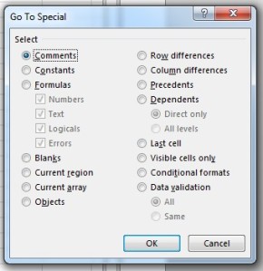
Alt + S	Opens the Go To Special dialog box from the Go To window
Ctrl + F	Opens the FIND dialog box
Ctrl + H	Opens the REPLACE dialog box

Note you can only use Alt + S after opening the Go To dialog box.

Go To is useful to get to cells or named ranges quickly. The Go To Special dialog box gives you the ability to navigate to or highlight certain types of cells in your worksheets such as any cells with conditional formatting applied to them.

The GoTo Special dialog box

Selecting/Inserting/Deleting/Hiding Rows/Columns

One thing you find yourself doing often is deleting or adding new rows and columns or wanting to hide some. So you end up right clicking and choosing from the options there or start searching for a button that can do it for you. I have found these to be quite useful little time savers;

Shift + Spacebar	Selects the entire row of the current selected cell
Ctrl + Spacebar	Selects the entire column of the current selected cell
Ctrl + +	Inserts cell(s) or a new row/column
Ctrl + –	Deletes cell(s) or a row/column
Ctrl + 9	Hides the row(s) of the selected cell(s)
Ctrl + 0 (zero)	Hides the column(s) of the selected cell(s)
Ctrl + Shift + 9	Un-hides the row(s) of the selected cell(s)
Ctrl + Shift + 0 (zero)	Un-hides the column(s) of the selected cell(s)

A few notes about this last set of shortcuts:

If you use Ctrl + +/- without selecting an entire row or column first then you get a dialog box asking you whether you want to insert or delete the selected cell(s) or the entire row or column.

Insert/Delete cell(s)/row(s)/column(s) dialog boxes

Also note that if you are using a laptop without a full numerical keypad, you need to use Ctrl + Shift + +/-. If these dialog boxes appear then press the letter key that matches your choice e.g. R to delete or insert an entire row.

So if you do want to use these keyboard shortcuts you are likely to do the following;

Ctrl + Spacebar > Ctrl + + which will insert a new column to the left of the selected column.

Using Ctrl + 9/0 will hide the row or column of the selected cell and if you IMMEDIATELY press Ctrl + Shift + 9/0 it will unhide whatever you just hid. However, it is more likely that you will want to unhide something at a later stage, so you will need to select the rows/columns either side of the hidden ones before you use this shortcut.

The final section is just a selection of other keyboard shortcuts I use, including some very basic ones that you can use in any application;

Ctrl + S	Saves the current document/workbook
F12	Opens the SaveAs dialog box
Ctrl + N	Creates a new document/workbook
Ctrl + C	Copies the selected cell(s) or object
Ctrl + V	Pastes the copied cells(s) or object to another location
Ctrl + X	Cuts the selected cell(s) to the clipboard
Ctrl + Z	Undo the last action (repeat for multiple undo actions)
Ctrl + Y	Redo the last action (repeat for multiple undo actions)
Ctrl + Shift + L	Applies AUTOFILTER to the selected cells/row
Ctrl + F1	Minimise/Maximise the Ribbon
F11	Creates a chat in a new chart sheet (uses default chart type)
Alt + F1	Creates an embedded chart in the same sheet (uses default chart type)
Shift + F2	Insert cell comment
F3	Opens the PASTE NAME dialog box to show a list of any named ranges you have in the current workbook
Ctrl + Shift + F3	Opens CREATE NAMES FROM SELECTION dialog box to create named ranges using existing column/row headings
F7	Runs spell check
Alt + F11	Opens the VISUAL BASIC EDITOR
Ctrl + `	Toggles between showing/hiding formulas in the worksheet (Note this is the combination on a UK QWERTY keyboard)
Shift + F11	Insert new worksheet to left of current worksheet
Alt + =	Insert the AUTOSUM function
F4	Toggle between relative and absolute cell references or repeat last action (limited use). See below for more information on the use of F4

After entering a cell reference in a formula press F4 to add in the “dollar” characters. Continue pressing F4 to get the required level of absolute/partial referencing.

Using the F4 button

And there you have 56 keyboard shortcuts that hopefully you will find a use for. As I said at the beginning this is not a definitive list. You still have about another 200 to learn beyond this list, but personally, these are shortcuts that I use regularly and cover what I think are the day to day actions that you will use in just about every spreadsheet you open.

PowerPoint – Creating Custom Graphics (Shiny Spheres)

Although there are lots of images you can download or copy from a variety of sources, sometimes you can’t find exactly what you want. The only way to get around this is to create your own custom shapes and images.
Although PowerPoint won’t ever have the functionality of Adobe Illustrator or Photoshop, with a handful of tricks you can create some fairly neat graphics to spruce up your presentations rather than stick to usual set of clip art or shapes available to you in the standard menu.
How about creating something like this…

What we are aiming to create…

Ok…a shiny sphere…what use is that? Let’s not forget that PowerPoint is there as an aid to presenting, not the presenter. Using abstract images or graphics can help to convey a message across rather than ram it down your throat. The explanation of the graphics is down to the presenter – after all it’s the presenter that the audience has come to listen to, not read page after page of bullet points (yawn!!).

So how do we create this marvel? I will show you two methods: one quick and simple, the other more involved and gives you more control over the end effect.

Method 1 – the more involved method:

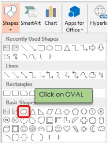
From the INSERT tab, select SHAPES and select the OVAL from the BASIC shapes section. Note that circles are not an option in Microsoft drawing tools.

Selecting OVAL to create a circle

To create a perfect circle hold down the SHIFT key while you drag the cursor, otherwise all you get is as the shape name suggests, an OVAL.

From the FORMAT tab go to SHAPE OUTLINE and remove the OUTLINE to your circle.

Remove the outline to a shape

Next we need to fill the circle with a GRADIENT FILL. Right click on the circle and select FORMAT SHAPE.

Then make the following settings:

1. Select GRADIENT FILL
2. Set the TYPE to RADIAL
3. Set DIRECTION to FROM CENTER
4. Make sure you only have 2 GRADIENT STOPS. Set a light colour at 0% (far left) and a dark colour at 70%. In this example I have used Blue-Grey, Text 2, Lighter 80% for the lighter colour and Blue-Grey, Text 2, Darker 50% for the darker colour. You can of course whatever combination you want.

I am using PowerPoint 2013 here but the same settings can be achieved in earlier versions too.

Now add a second smaller OVAL/CIRCLE on top of your first circle. You can use either a circle or an oval, your choice, whichever you think looks best. I will add an oval in this example.

Again you will need to apply similar settings to your first circle…no outline, gradient fill etc. but this time with slightly different setting on the GRADIENT FILL.

Settings for the smaller sphere

1. Set the TYPE to LINEAR
2. Set DIRECTION to LINEAR DOWN
3. Set the first stop (far left) to WHITE and use the same dark colour as before for stop 2 but this time set it to 80-85%
4. Set TRANSPARENCY to 100%

The final step is to add a SHADOW under the sphere.

Click on the main circle (you don’t want to create a shadow for the smaller one), then right click and select FORMAT SHAPE again, but this time pick the EFFECTS section and select SHADOW. Go for any setting you like. In this example I have used the following settings:

Shadow settings for your sphere

Method 2 – the quick and easy way:

Create your circle, removing any shape outline, exactly as outlined in the steps above.

On the FORMAT tab look at the SIZE of your circle and make a note of the size shown.

Size of your shape

Now right click on your circle and select FORMAT SHAPE. Go to 3-D FORMAT and set both the TOP and BOTTOM BEVEL to ROUND.

Bevel setting

You now need to set the WIDTH and HEIGHT values. To set this correctly and quickly, you’ll need the size of the circle you created. To calculate the correct values for your circle you have to do a quick calculation;

• If working in centimetres – diameter x 14
• If working in inches – diameter x 36

Apply the calculated number to width and height for both top and bottom bevels. So using my example here, the values would need to be set to 9.22 x 14 (my laptop works off metric measurements) to give a value of 129.08, which I have rounded down to 129.

The end result then looks like this;

                               Quick sphere

This gives a perfectly acceptable result and creates a complete sphere that you can rotate which changes the lighting slightly across the surface.

Whichever method you choose to use, you can create as many of these as you like in any colour you like to match your presentation theme.

Spheres in various colours. With a bit of added animation you can turn these into a Newton’s cradle!

How you then choose to design your own graphics is entirely up to you and the message you are trying to get across to your audience.

Using spheres with some added 3-D images

Although this sort of thing takes time, the end result is worth it, and with practice it takes less time, and ultimately you can move away from the standard dull/unimaginative bullet point/clip art type presentation that send people into a presentation weary comatose state. Even if they don’t think the topic is interesting, at least they might show some interest in your amazing graphics!

Now go and get creative.