Excel: Text Functions (Part 2)

Continuing from my last blog, here are the remaining text functions I have found useful:

LOWER

Syntax: =LOWER(text or cell ref)

This will convert any characters in UPPER case to LOWER case. Your immediate thought will probably be ‘when am I ever going to need that?’, but people enter data into your spreadsheets all in lower case or upper case or some weird illogical combination of both, and so to give your text values some sort of uniform appearance, this sort of function comes in handy. You will most probably use this in combination with other text functions.

UPPER

Syntax: =UPPER(text or cell ref)

This gives you the opposite to the previous function, converting all LOWER case characters to UPPER case. As with LOWER, you will probably use it in combinations with other functions.

PROPER

Syntax: =PROPER(cell ref)

A function of limited use really, and probably limited to using with names. This one capitalises the first letter of every word in a cell. This can be useful when working with names that have been entered in some haphazard way…

…but avoid using with sentences or blocks of text.

Not pretty!

FIND

Syntax: =FIND(what to find, cell ref)

Another text function which on its own is of little interest but works best when combined with other functions. Basically it gives you the position (reading from left to right) of whatever it is you are trying to find. If you try finding a text string (i.e. multiple characters or even a word) it will give you the position of the first character or digit of what you are trying to find.

In column B, I am looking for the dash (-) and in column C, looking for the text string “Sm”. Not really of much use until combined with other functions to be honest but check out the combinations section further on for some examples. Also note that it will only give you the position of the first instance it finds starting from the left.

EXACT

Syntax: =EXACT(cell ref 1, cell ref 2)

Basically, this tells you whether contents of two cells are identical or not. Another one that is best used in combination with other functions, testing values before they are manipulated in some way.

In column B, I am looking for the dash (-) and in column C, looking for the text string “Sm”. Not really of much use until combined with other functions to be honest but check out the combinations section further on for some examples. Also note that it will only give you the position of the first instance it finds starting from the left.

SUBSTITUTE

Syntax: =SUBSTITUTE(cell ref, old text, new text [,optional instance number]))

Whereas REPLACE replaces everything that meets your criteria, SUBSTITUTE gives you the choice to (effectively) replace every instance of your criteria or a specific instance i.e. the 2^nd or 3^rd time etc. that it appears in the cell. Let’s say our part number has been changed where the 2^nd dash needs to be substituted with a forward slash. This function, has quite a specific use and may not be one you will use on daily basis, but it is worth knowing and as with most functions works best in combination with other functions.

REPT

Syntax: =REPT(“character/letter/symbol”, number of times to be repeated)

In terms of functions, this one ranks amongst one of the most pointless….but it can come in very handy to create a fake chart! Basically you pick a character and work out how many times you want to repeat it in a cell.

Sparklines in 2010 have made this a tad redundant but can still be quite effective for a quick chart effect, and you can get creative using Wingdings or Webdings as well as apply conditional formatting! Awesome!

And then it’s all about putting them together in various combinations to extract and modify text…

Other functions in the TEXT category that may be of interest but personally have either never used or used just once for a very specific job are;

REPLACE – replaces characters but you are more likely to use CTRL + H and use the replace dialog box.

CHAR and CODE if you need to generate random characters based on their code, or to work out the code for a given character e.g. A= 65, a = 97……85 = U.

SEARCH returns the position of a specific character (reading from left to right) within a text string specifying from which point you want to start searching.

TEXT allows you to format a value into a specific text format which of course means you can no longer perform calculations on that value.

VALUE is TEXT’s counterpart converting numbers formatted as text into numerical values.

So that’s TEXT functions in Excel, but as I have mentioned a few times, the power of these functions really comes through when you combine them together. Here are a few examples, but how many and how you combine them will depend entirely on your own requirements…

1. =UPPER(LEFT(TRIM(A2),3))Removes any leading/trailing spaces, extracts the first 3 characters starting from the left and then converts them into upper case.
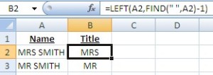
2. =LEFT(A2,FIND(“ ”,A2)-1)Works out the position of the first space in the cell, takes away 1 from that value to give you the position of the last character before the space and extracts all characters up to that point.

   

3. =IF(LEFT(A4,1)=”T”,A4,E4&”.”&D4&”@”&F4)If the first letter is a “T” then display that value, otherwise join a number of cells together adding a dot and an @ sign to make up an e-mail address.
4. =SUBSTITUTE(IF(ISERROR(LEFT(A2,FIND(“@”,A2)-1)),A2,LEFT(A2,FIND(“@”,A2)-1)),”.”,” “)This checks the cell contents to see if there is an @ symbol. If not (in this example…if the test produces an error) display the contents, but if no error is generated take all characters to the left of the @, and then replace any dots with spaces.

So now it is just a case of experimenting with different combinations. If you are not confident nesting functions then build them up a bit at a time. Let’s take the first combination example:

=UPPER(LEFT(TRIM(A2),3))

Think about the problem logically to apply the functions in the correct order:

• Remove any spaces that may or may not be there so we TRIM first as we don’t want to start counting characters before we remove any chances of counting spaces or non-printable characters.
• Then what do we want to extract? So now we can apply the LEFT function to the output of the TRIM function.
• Finally, we want to convert whatever comes out of that into UPPER case.

So apply one function at a time, make sure it works at each stage with each additional function. If you try to do it all in one go, chances are you’ll only confuse yourself and end up ‘correcting’ things that are fine and making things worse. With experience you will be able to string these together in next to no time.