Excel – Protecting Your Worksheets and Workbooks

Having spent a lot of time creating the perfect workbook, setting it just how you need it ready to do other important work, you send it out to people around the office or business, or perhaps you place it on a shared drive for everyone to access, only to find that within days, or even hours, some bright spark doesn’t like your layout and changes it around to suit them regardless of the fact that it was set up in a particular way for a specific reason.

This is where we need PROTECTION.

To protect a workbook there are number of steps to follow:

1. Unlock any cells that the user(s) need access to – this will apply to all visible sheets.
2. Protect any sheets users will have access to, and hide any sheets users don’t need access to.
3. Protect the workbook itself

A quick word first about the effectiveness of protecting workbooks. Basically, it’s not very secure. There is software readily available for free off the internet that will quickly hack into a workbook – I use one myself by Rob Bovey at www.appspro.com called Excel Utilities v.7 (check out my video on WordPress/YouTube – “Clearing Workbook & Worksheet Passwords” showing how well it works http://wp.me/p2EAVc-3u).

You’re probably thinking “so what’s the point of protecting my work if someone can hack into it so easily??”, but in the majority of cases, especially in the work environment, many companies don’t like or even allow the use of freebie add-ins off the internet and to be fair, most people couldn’t be bothered hacking into a workbook at work…..why create more work for yourself?

Step 1: Unlocking Cells

When you open the FORMAT CELLS dialog box you may have noticed a tab on the far end called PROTECTION.

The protection tab in Format Cells

You may have tried ticking and unticking the options and seen no difference whatsoever to your spreadsheet, but notice the comments below the tick boxes – “Locking cells or hiding formulas has no effect until you protect the worksheet”. However, this step is vital once protection has been applied to control what people have access to in the worksheet.

All cells, by default, are locked. Therefore, select ALL cells that you want people to be able to edit or fill in and untick the LOCKED option. Any cells you don’t want people to change or enter information into, leave as is – locked!

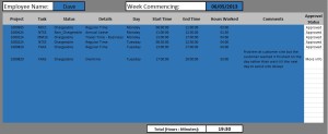
Using our timesheet example that we used to create VALIDATION rules, the cells highlighted in blue have been unlocked in preparation for PROTECTION.

Once you are satisfied that all the correct cells have been unlocked go on to step 2…

Step 2: Protect Your Worksheets

Before protecting every sheet in the workbook, stop and think about which sheets people actually need to use and/or see. For example, you may have a sheet where all the lists that are used in your DATA VALIDATION lists are kept. Do people need to see those? Probably not. So rather than set up a password etc. to protect the sheet, hide it instead. Do the same for any other sheets that people don’t really need to see or access. Protecting the workbook in step 3 will prevent people gaining access to all your hidden worksheets.

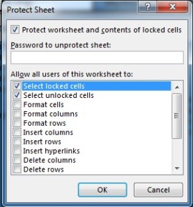
Go to the REVIEW tab and click on PROTECT SHEET.

In the following dialog box you have the option to create a password. Personally I don’t set a password until I have tested everything to make sure it works how I want it to. If you set a password while still testing, it just means you have to type in the password every time you want to make a change and reset it again afterwards. A minor pain….your choice.

You can also decide what freedoms you are going to give to your users. Do you want people to be able to add or delete rows or columns etc.? The only option you must leave ticked is SELECT UNLOCKED CELLS. If that is unticked, you can’t even select the cells you want to edit!

Test your settings. Can you get to all the cells that need to be filled in or edited? Are all the cells you want to block access to safely locked? Lock or unlock cells as appropriate and re-test.

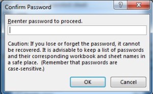
Once fully tested and working OK, set a password, confirm the password in the next dialog box and click on OK.

Now that the worksheet(s) are protected you’d think that would be enough. A lot of options, including DATA VALIDATION have been made inactive and appear greyed out in the ribbon.

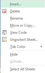
However, if you right click on any of the worksheet tabs you can still rename, delete and move worksheets.

To deny all access to this you now need to complete step 3 – protecting the workbook.

Step 3: Protect Your Workbook

Click on your REVIEW tab again, and click on PROTECT WORKBOOK.

Protect the workbook, with or without a password, and test it. Try to delete or rename sheets, try to get to validation lists etc. Make sure you check EVERY sheet. Protecting a workbook does not give any cell protection to a sheet that has not been protected, leaving users free to edit any content on that sheet.

Once fully tested, apply passwords and you are ready to unleash your workbook on the world.

Unless you have Rob Bovey’s Excel Utilities and the break passwords function (or equivalent) DON’T FORGET YOUR PASSWORDS! Making copies of the workbook or other similar tricks won’t work – it will copy all the passwords across at the same time.

As an optional extra, you can also apply protection to individual cells or ranges of cells that require a password to gain access.

Let’s take out timesheet example again. We have unlocked all the cells that people need access to, but there is a column called “Approval Status”. This is where a manager has to approve/reject the line recorded in the timesheet. If I leave this unlocked, then the person filling in the timesheet would have access to these cells and self-approve their timesheet.

By leaving this set of cells locked, the general user cannot access them, but I need the cells to be accessible by the manager. For that, I can use ALLOW USERS TO EDIT RANGES.

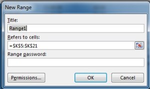
Select the range of locked cells and on the REVIEW tab, click on ALLOW USERS TO EDIT RANGES. Click on the NEW button on the dialog box that appears. On the next dialog box give your range a TITLE (e.g. Approvers). If you have highlighted the cells, the REFERS TO CELLS box should show the cell range. If not, simply click on the range selector button and highlight the range you want. Finally set a password, confirm it and click on OK.

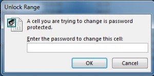
Now if anyone tries to type into one of these cells they will be prompted for a password.

So with a combination of validation rules and protection your workbook should be fairly safe from interference from the majority of people.

Excel – Using Formulas for Simple Double Entry Bookkeeping

Do you require people to fill out a sheet such as expenses in a simple double entry format, but find that people add the costs to all the wrong columns? There is a simple way to control this with a combination of a formula, data validation and a bit of protection.

Let’s take a simple example;

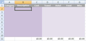
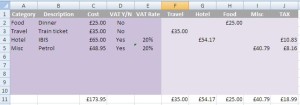
People put in expense claims for the following categories: Travel, Hotel, Food, Misc

For each expense they need to add a short description and a value. The value then needs to be added to the correct column across the page, in effect creating a double entry table.

The problem of course, is getting people to correctly add the value to the appropriate column and to make sure that all the columns add up correctly to match the grand total in column C.

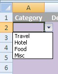
First of all, control the category column. Add a data validation list based on the column headings and limit the list to those values.

Add some standard currency formatting to your various monetary cells.

Now add a formula to auto-populate the correct columns once they have selected a category and entered a cost.

The formula to use here would be:  =IF(EXACT($A2,D$1)=TRUE,$C2,””)

This will test to see if the category selected in column A matches the column heading in columns D to G. If they match then it displays the value in column C, otherwise leaves the cell blank.

Note, that until a value is entered in column C it will display £0.00, which is fine as it flags an incomplete cost and should prompt the user to enter a value.

The final step is to protect and lock columns D to G to prevent users randomly entering data in these cells. Make sure the cells in columns A to C are unlocked to allow editing once protection is applied.

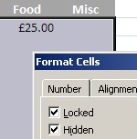
Make sure that the cells in columns D to G are both locked and hidden so that users cannot see the formulas (not essential but adds to the magic of the worksheet). Add a password to prevent users making changes and make sure you protect the workbook too to prevent anyone from removing the sheet or making changes to data validation rules etc.

Now when a user adds in their expenses, the values are automatically added to the correct column and because people cannot randomly add or edit values the totals for each column will add up to the grand total of all the expenses claimed.

From here you can extend your formulas to calculate net cost and VAT where applicable, and get those to automatically calculate based on selections I’ve now added to columns D and E.