Excel – Basics of Pivot Tables

If you are familiar with Pivot tables then you will know just how amazing they are. If not, then read on.

Knowing how to use Pivots is one of the MUST KNOW features of Excel. Since Office 2010 there has been a new add-in called PowerPivot which takes the humble Pivot table and turns it into an all singing and dancing monster of a BI tool. This blog will look at the basic Pivot table, but don’t despair, this is a very powerful tool in its own right, and if you have to analyse data on a regular basis this is the tool for you.

Are you the sort of person who dreads month end reporting? Your boss gives you a huge file and asks you to run through it and asks for some sort of analysis to show what’s happened in the last month/quarter etc. and of course expects it in next to no time because apparently it’s quite simple and quick to do.  If that were true then;

1. Your boss would be able to do it
2. It wouldn’t take you several hours or even days of stress to get even close to what is required

This blog will show you how to reduce this time frame down to a matter of seconds to produce a summary report/analysis using a Pivot table.

First of all…some pre-requisites in order to be able to use a Pivot table;

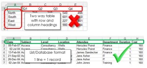
• Your data must be in a LIST or DATABASE format. In other words you can only have columns of data with NO ROW HEADINGS. Each row of data is a distinct record.
• Each column must have a unique HEADING and there must be no completely empty columns within your data table. You can have an empty column as long as it has a heading (not that that is very useful…but it will work)

Dos and don’ts of data to build a pivot table

As long as your data meets these basic requirements then you are good to go to build your Pivot table.

Before we create a Pivot table…let’s look at what it does.

If we look at some very basic data, we can see a number of people, the regions they work in and the sales they have achieved.

Excel will look down each column and will “group” the labels it finds. So in the salesperson column it will group all the names together to create a list of unique values. It will repeat this in each column that is selected to be part of the Pivot table. So in this example, if we look at Bob we can see that Bob appears 3 times in two regions. The Pivot table grabs all the information and will group, count or sum up any values associated with Bob in each region. So in the end result we can see that Bob has total sales of 912 in the North and 326 in the South. Depending on which columns you select and perform summary calculations on, the Pivot table will “group” all the relevant labels and values to give you an instant summary of your data table. This grouping effectively allows you to convert a list into a two-way table and to review and analyse data in almost any number of ways.

How a Pivot groups information

Now that we have a basic understanding of what the Pivot table can do, let’s create one.

Click anywhere in your data table.

Go to the INSERT tab, and click on PIVOT TABLE in the TABLES group. You will notice there is a RECOMMENDED PIVOT TABLES in Excel 2013. I will mention those a bit further on.

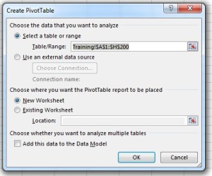
You will then see this window;

The create pivot table window

If you were clicked somewhere in the data table it works out the boundaries of your list and automatically populates the TABLE/RANGE information. If you weren’t in your table then click on the selector button and manually select the data range. Alternatively, if you use named ranges type in the range name.

Decide where you want your Pivot table to appear – NEW WORKSHEET or in an EXISTING WORKSHEET. If you opt for EXISTING, click on the range selector button and select a cell somewhere in your workbook. The cell you select will be the top left hand cell of your Pivot table area. Make sure that you leave enough room to the right and below to ensure the Pivot table does not overwrite any existing data. If an overlap is detected, then you should see this message box appear:

Warning – overlap of Pivot and existing data

I would suggest at this point to select CANCEL and choose somewhere else to start your Pivot table from.

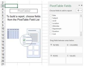
You will now see two new windows appear;

Build your Pivots area

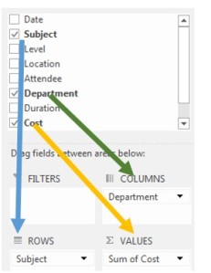
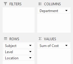
Click and drag the column or FIELD names from the top window into the appropriate area in the grid below the list.

Click & drag field headings into your Pivot building grid

You are not limited to one field per segment in the grid, you can have as many as you have actual field names available…although that can start to look messy and can make your Pivot table difficult to read.

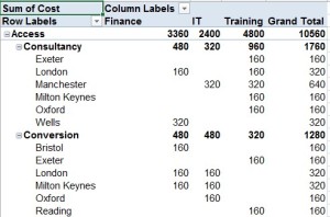
Here’s an example of multiple row fields being selected;

Multiple Row values added

Pivot showing multiple fields added in

The great thing about Pivots is that if you don’t like the end result or prefer a different layout you don’t have to start again. Just click and drag fields from one area to another or remove them completely and add new ones until you get the type of table you need.

Something to note:

• By default anything you put in the VALUES area will have the SUM or COUNT function applied to it. If the data you put in this area contains numbers and no blanks it will automatically use SUM. If the data has blanks or contains TEXT values then it will apply the COUNT function.

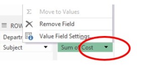
You can change the summary function to any fields sitting in the VALUES area by clicking on the little arrow next to the field name;

Getting to your Value Field Settings

Then click on VALUE FIELD SETTINGS.

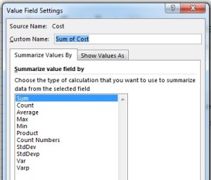
Pick a calculation method from the SUMMARIZE VALUE FIELD BY list.

Changing the summary calculation method

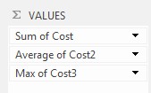
You can drag the same field several times into the VALUES area and apply a different function to each instance.

Field name plus a number to create a unique label

In this example I have applied the SUM, AVERAGE and MAX functions to the same field (Cost). Notice how it has named them Cost2 and Cost3. This is because when you add a field several times, it will apply the default the summary calculation first (SUM or COUNT) and as Pivot tables can only work with unique field names it adds a number to any repeated field names in the VALUES area to give each one a unique name. As you apply the new function it will change from SUM or COUNT to whatever function you have selected.

You can create as many Pivot tables as you like off a single data table, meaning you can summarise your data in a variety of ways. If you are moving from Excel 2003 or earlier you will no longer be prompted about using the same cache or a new one. All Pivot tables since 2007 are created using the same Pivot cache if the same data list is used each time.

If you are wondering what a Pivot cache is, it’s a virtual copy of your data list that is automatically created when you get past the Create PivotTable window and sits inside the workbook as a virtual data table. It’s important to understand a little bit about the cache.

Your Pivot table is not directly linked to your data list. When you first create a Pivot table it takes a snapshot of your data and stores it in the cache. Your Pivot table then interacts directly with the cache. The downside to this is that as this cache is a snapshot in time of your data. If you update/edit any data in your table, it means the cache is no longer the same as it is frozen in time when the pivot was set up (that could be 10 seconds ago or 1 week ago!). To update the cache, simply right click anywhere in your Pivot table and select REFRESH. Your Pivot table will now update itself showing the latest data values. And because you can have multiple Pivot tables all running off a single cache, ALL the tables linked to that cache will update at the same time.

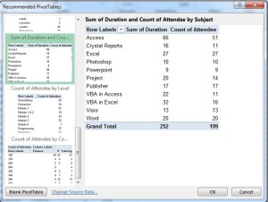
At the beginning I mentioned RECOMMENDED PIVOT TABLES which was a new  feature in Excel 2013. Basically, Excel looks at your data using the field names it makes a number of suggested layouts.

Recommended Pivots from Excel 2013

Pick the layout that suits your needs and click OK. Job done! Although this is quick and easy (i.e. requires virtually no thought) I would still try to create a Pivot table manually…as you’ve seen, it’s not that difficult, and by doing it manually you get exactly what you want…the choice as they say, is yours!

And that is how you create a basic Pivot table. As you get used to clicking and dragging fields into the various ROW/COLUMN/VALUES areas you will find that you can create a Pivot table (on familiar data) in 5-10 seconds…flat! And if your boss does not like your initial layout, click and drag the fields until they are happy. Each change will only take a matter of seconds so gone are the hours or even days of stressing over those month end reports.

In other blogs I will show you how to use the REPORT filter, customise your Pivots, create Pivot charts, group data and add calculated fields….to name but a few of the wondrous things that Pivots can do.