Excel VBA – Event Procedures

Most of the time when you write a macro, it’s one that you will run by clicking on a button on the Quick Access Toolbar, or from a button on the Ribbon, or even directly within your Visual Basic Editor. Whichever method you use, the code is running on demand.

If you write code that other people may end up using, from a workbook on a shared drive for example, relying on users to run code is very much hit and miss. Some will be reliable and click on the right button at the appropriate moment. Others…..forget it.

So how can you force the user to run code at the right time?

What you need is an EVENT PROCEDURE. Unlike a normal sub routine that has to be manually kick started, an EVENT PROCEDURE automatically runs if the user does something within your workbook.

EVENT PROCEDURES take place at either workbook or individual worksheet levels within a workbook. The types of events vary at each level.

When you look at your PROJECT EXPLORER window you will see the names of any sheets in the workbook as well as something called THISWORKBOOK.

Finding ThisWorkbook in the VBA Editor project explorer window

It is here, in either (or both) at worksheet and/or workbook level that you will add your EVENT PEOCEDURES, not in modules as you do with normal sub routines.

Let’s start with WORKBOOK level procedures.

Double click THISWORKBOOK. This will open a blank sheet to write code, but we don’t want to use this. Click on the drop down on the right hand side above the work area and select WORKBOOK.

Getting to the Workbook scripting area

After clicking on WORKBOOK you should see this;

Default event at Workbook level

The editor automatically selects an event. Nothing you can do about this. It doesn’t mean you have to do anything with this, it’s just the default event to appear at workbook level.

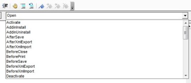
There are a number of events that you can choose from. To see the full list go to the top right hand corner and click on the dropdown.

Workbook level event options

Use the scrollbar to view all the events available to you at Workbook level.

There are also events that run at WORKSHEET level. Double click on any of the sheets in your workbook and you get a blank sheet for code, identical to what happened when we wanted to create an event at workbook level. Where it says GENERAL, click on the drop down and this time select WORKSHEET.

Selecting Worksheet level

As with WORKBOOK events, the editor will display a default event. In the case of WORKSHEET it’s SELECTION CHANGE.

Default event at Worksheet level

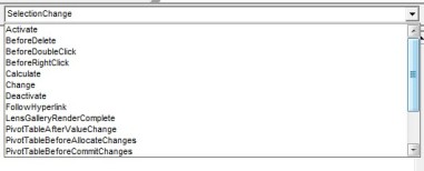
If that’s not the event you want, click on the drop down on the right hand side where you can see SELECTION CHANGE. There are not as many options at this level as there were at WORKBOOK level, but still enough to keep you entertained.

Worksheet level event options

Again, use the scroll bar to see all available options.

Whether it is an event at WORKBOOK or WORKSHEET level, simply add your code as normal. Unless you know your events inside out and the variables they require, don’t try to get creative editing the opening line i.e. Private Sub… into the event you want. Pick the event you want from the drop down list and delete whichever one you don’t need from the editor sheet. If you try to edit the opening line, chances are you’ll dig yourself into an extremely deep hole from which you will probably never escape.

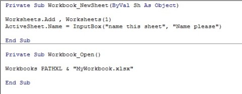
The most common mistake people make when starting to use events is to type in a command line that does the event. If you are not sure what I mean here are a couple of typical mistakes as examples;

Typical event errors by beginners

In a workbook called MyWorkbook the user wants something to happen when they open it. Unfortunately,  a line has been added that opens the very book they just opened. Don’t do it.

On a NEWSHEET event, whenever a user adds a new sheet, the code then adds yet another new sheet to the workbook and prompts the user to name this sheet rather than the one the user added.

Now…these two may seem like minor issues, but you don’t need to write an action to do what has already happened. Remember, it is the opening of the workbook by the user that triggers some code, so there is no need to write code that opens the workbook that has just been opened. In the same way, when someone clicks on the NEW SHEET button or right clicks and selects INSERT, you don’t want to add yet another blank sheet…the user has just created the event that triggers some code to run.

By all means, when a workbook is opened, open one or two more as these may be required. Effectively, you are making sure that the user is provided with all the workbooks they need to complete a task, and therefore eliminating any risk that the user forgets to open the others.

And that is really what you are doing with events in many cases – eliminating risk;

• Before closing a workbook make sure a copy of the workbook is saved in the correct folder in the correct drive
• Before saving changes to a workbook make sure all cells that need to be filled in have been
• If a new sheet is added, or a new version of a workbook is created, set the correct naming convention for sheets and workbooks etc. the possibilities are almost endless

An interesting example is one by Tom Urtis, getting a workbook to delete itself. http://www.atlaspm.com/toms-tutorials-for-excel/toms-tips-for-excel-workbook-suicide/

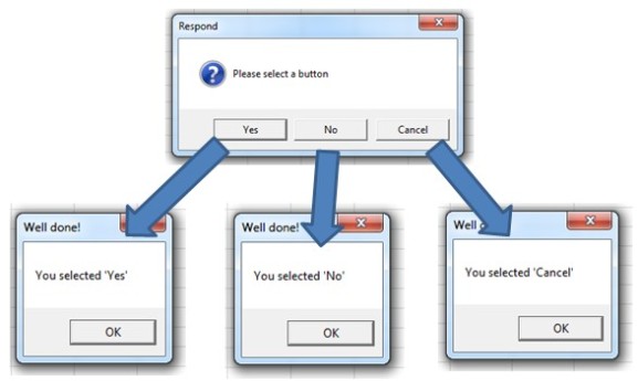
Or if you want to have a bit of fun and annoy people, try this;

VBA fun…strictly for geeks 😉

Highly annoying!

So don’t be afraid of using EVENT PROCEDURES. They can be very useful (ignoring the annoying example above) and can ensure that what you want to happen with your workbook actually does, without having to rely on users remembering to do things, which more often than not, doesn’t happen.

 

Excel VBA – Automatically Close an Inactive Workbook

A big problem I’m sure many of you have encountered is being locked out of a workbook saved on your network because someone is in it, or more likely, has opened it and forgotten to close it when they’ve finished. There may well be a message giving you some user ID or some other vague name of the person who is currently in the workbook but you have no idea who that person is, whether they are on your floor or even in the same building. Even if you can work out who they are, chances are they are not at their desk and the computer screen is locked. So you end up simply waiting to see if the workbook is ever freed up and praying that no one else beats you to the released workbook.

So what are your alternatives?

You could opt to have a shared workbook allowing multiple users to access it at the same time. This can work, but someone has to take overall ownership of the workbook to agree changes and any conflicts that may arise within the workbook between users. There are also restrictions applied to some of the functionality within a shared workbook, such as not being able to add or modify data validation rules. Some of the lost functionality will definitely add restrictions that may make the workbook unworkable for many people. Check the Microsoft website for a full list of what you can’t do in a shared workbook (https://support.office.com/en-us/article/Use-a-shared-workbook-to-collaborate-79bd9dee-1aa3-49b5-bc27-a1ad28ffcbce?CorrelationId=4365b78b-4666-4d41-adcb-32c850345466&ui=en-US&rs=en-US&ad=US#__excel_features_that)

Another option is to keep the workbook “un-shared” but make it close itself down after a set period of inactivity. Like that, if someone does walk away from the workbook without closing it or simply has it open despite having finished whatever they were doing, a built in timer detects that nothing has happened and automatically closes the workbook so someone else can get in.

In order to do this we are going to need a bit of VBA code.

We will need 3 routines to start with (the name I will give to each routine is shown in brackets…feel free to call yours whatever suits you best);

1. Start the timer (StartClock)
2. End the timer (StopClock)
3. Close the workbook (ShutDown)

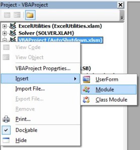
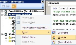
Open the Visual Basic Editor (Alt + F11) and find the workbook you want to automate. Right click on it and select INSERT and then click on MODULE.

Adding a new module

The three routines we need to make all this work need to be created here so they can be called on by event procedures we will create a bit later.

We will need a global variable to store the time each time any of the routines start up. At the top of your module (in General Declarations) declare a PUBLIC variable so it can be recognised anywhere within our project/workbook.

Public NoActivity as Date

The first procedure we will create is to close the workbook and save any changes that have been made to it (you could also choose to not save changes to prevent half-finished data from populating your spreadsheet).

Sub ShutDown ()

Application.DisplayAlerts = False

With ThisWorkbook
.Save
.Close
End with

End Sub

Here we turn off any warning messages in case any pop up, save any changes and then close the workbook. If you don’t want to save any changes you can use .SAVED = TRUE to replace .SAVE.

Sub StartClock ()

NoActivity = Now + TimeValue(“00:05:00”)

Application.OnTime NoActivity , “ShutDown”

End Sub

Here, we populate the variable with the current time plus whatever period you have decided is your limit for inactivity. In this example I’m setting it to 5 minutes.

ONTIME says when we reach now plus 5 minutes, run the SHUTDOWN routine

Sub StopClock ()

On Error Resume Next

Application.OnTime NoActivity, “ShutDown”, , False

End Sub

In this routine, in case anything goes wrong ignore it, and once again if the time limit is reached run the SHUTDOWN routine. The FALSE bit is just there to clear any previously set procedure.

Now that our three routines have been created, we now we need to create some event procedures that will trigger these routines.

If you are unfamiliar with EVENT PROCEDURES, they are routines that start automatically when something happens in the workbook such as the user selecting another sheet. With an EVENT PROCEDURE you are not relying on the user to press a button to run a routine, it simply happens automatically when triggered by an event in the workbook or worksheet.

Double click on ThisWorkbook in the Microsoft Excel Objects folder of your workbook.

Accessing events on ThisWorkbook

Then, from the left drop down box above the script area, select WORKBOOK.

Selecting the Workbook area to add events

The editor automatically adds the OPEN event, which in this case is one of the events we need.

In the event add the code CALL STARTCLOCK;

Private Sub Workbook_Open()

Call StartClock

End Sub

Now, whenever the workbook is opened, the STARTCLOCK routine starts and therefore the timer starts. It may be worth adding a message box here too to warn users that the workbook will automatically close after x minutes of inactivity.

In terms of events that mean the user is doing something in the workbook, we want the following events to restart the timer;

Workbook_SheetCalculate

Workbook_SheetSelectionChange

Might be worth adding this event at worksheet level to stop the timer if people are just browsing in the workbook rather than editing…it is still a form of activity…albeit unproductive!

Worksheet_SelectionChange

And we need a final event to stop the timer just before closing the workbook;

Workbook_BeforeClose

So all our event code will look something like this;

Private Sub Workbook_BeforeClose(Cancel As Boolean)

Call StopClock

End Sub

—————————————————————————————————————————

Private Sub Workbook_Open()

MsgBox “Please note that this workbook will close,” & vbCr & _
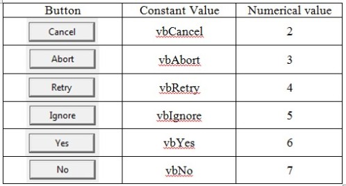
“saving any changes you have made after 5 minutes of  inactivity”, vbInformation, “Warning”

Call StartClock

End Sub

—————————————————————————————————————————

Private Sub Workbook_SheetCalculate(ByVal Sh As Object)

Call StopClock

Call StartClock

End Sub

—————————————————————————————————————————

Private Sub Workbook_SheetSelectionChange(ByVal Sh As Object, ByVal Target As Range)

Call StopClock

Call StartClock

End Sub

Next time you want to post a workbook on a shared drive at work, you now have the following options:

• leave the workbook as it is and hope that people are sensible and close it when they are done
• set it up as a shared workbook, accepting whatever restrictions this imposes
• create a workbook with its own built in shutdown mechanism if nothing happens within a set timescale.

If you want to download a copy of the workbook with this code in it, then follow this link – https://onedrive.live.com/redir?page=view&resid=2C036E200F2C8BCF!255&authkey=!AI887S1-lcOY6RU

 

Excel – Introduction to Recording Macros

In this blog, I am going to introduce the concept of macros in Excel, and show you how to record and run basic macros – if you already write your own code, then read no further.

Macros are a great feature in Excel (and any other Microsoft application for that matter). They are simply a series of steps which have been automated. So instead of you clicking several buttons, or highlighting data and formatting it in some way, a macro can complete all of those actions with the single click of a button – so they are potentially huge time savers.

The recording of macros is very simple, but it is limited, and ultimately, if you want to automate your work in Excel you need to write code from scratch.

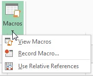
The simplest way to create a macro is to record it. You can do this via the VIEW tab and click on MACROS, and select RECORD MACRO.

Although you can access everything through this button, I would recommend turning on the DEVELOPER tab. This give you access to more things relating to macros and VBA as well as form controls. If you’re using 2007, click on the OFFICE button and click on EXCEL OPTIONS. From the POPULAR tab tick the SHOW DEVELOPER TAB IN THE RIBBON option. For those on 2010 or 2013, right click on the RIBBON, select CUSTOMIZE THE RIBBON and tick the DEVELOPER box in the right hand window.

Time to start recording…

First of all plan what you are about to record. I say this because the recorder records everything you do…including mistakes, re-edits etc. It just means that every time you run the macro it will repeat all the mistakes and the consequent corrections (albeit at high speed), so plan and if necessary do a couple of practice runs so you know which command/icon to click on, what to select etc. The recording is not done in “real time”, so if you pause to answer the phone, or have a cup of tea in the middle of your recording it won’t record several minutes of inactivity. It only records actions on screen, and an important thing to bear in mind here, it records ONLY the actions you perform in Excel. Opening Windows explorer, or Word or anything else for that matter will not be included as part of the recorded macro. Remember, I said it was limited.

Assuming I have planned and rehearsed where necessary, it’s time to do the actual recording.

Click on the VIEW tab, MACROS, RECORD MACRO, or go to the DEVELOPER tab and click on RECORD MACRO.

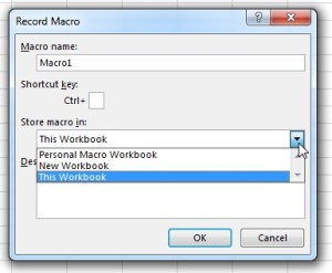
You should then see the following window;

Give your MACRO a NAME. Using the default name is fine, but once you have a collection of macros all called Macro1, Macro2 etc. it will be very hard to tell one from another unless you look at the code to work out what each one is doing. So give it a helpful name. Note that no spaces are allowed in macro names. If you do want a space of some sort, use an underscore (_). Personally, I use something that is called Camel Hump Text i.e. capiltalise the first letter of each word that makes up the name of your macro. YouWillBeSurprisedAtHowEasyReadingTheNameIsDespiteBeingContinuousText…I rest my case.

The choice as always is down to your own personal preference.

You can assign a shortcut key to your macro. All I will say here is “good luck” finding a free combination of keys. Easier to just add a button to your Quick Access Toolbar or create new tabs on your Ribbon (2010+) and add buttons there.

Now for the important bit: STORE MACRO IN. You will be presented with 3 options;

1. Personal Macro Workbook
2. This Workbook
3. New Workbook

If the macro is going to work exclusively in, or from within the current workbook, then select THIS WORKBOOK. So if the macro is unique to the current workbook and won’t be used elsewhere or the macro (for example) imports data from other sources, but ultimately does all the work in the current workbook then THIS WORKBOOK is the best choice.

NEW WORKBOOK is a bit of a pointless choice in my opinion as the new workbook effectively becomes the new THIS WORKBOOK. End result is same as above.

If, however, you want your macro to work in any workbook at any time, or it involves opening a workbook for example, then the best place is in your PERSONAL MACRO WORKBOOK. This is a blank workbook that sits in the background to Excel and is used purely to store your macros in “folders” called MODULES. By default, PERSONAL does not exist, you need to record something in it to get it kick started. Once created, you can either record or write code directly inside the modules. PERSONAL, is as the name suggests, personal to your Excel. It resides on your computer alone.

If you choose the “wrong” place by mistake you can easily copy/cut and paste code from one workbook to another (assuming PERSONAL has been created).

The final box is for comments. This serves no purpose other than to add a note to say what the macro can do or just some information that may be of use to you or any other user of the macro.

Click on OK to start recording.

Do whatever it is you need to do, and remember to STOP RECORDING once you have done . Click on STOP RECORDING in the DEVELOPER tab or the small square in the bottom left hand corner of the screen.

 

or

 

 

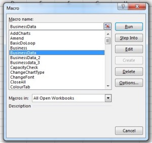
To run the macro you have just recorded, go to the DEVELOPER tab and click on MACROS, click on the macro name and then click on RUN.

As this is quite a long winded way of running a macro, add a button to your Quick Access Toolbar (QAT) or add a new tab to the Ribbon.

Here is a quick video showing a macro being recorded and a shortcut button added to the QAT.

If you want to view the code that has been recorded then go to the DEVELOPER tab and click on VISUAL BASIC or use ALT + F11. This will open the Visual Basic editor. Take a look at the code. It’s not as difficult to decipher as you may think –

• Font.Color
• Cells.Select
• Font.Bold = True

Without knowing any code, these sort of bits of code are self-explanatory. You may not know the details or the why but you can get a pretty good idea of which bit does what in your recorded code. Like any language, you need to practice it to become “fluent” and VBA is no different. The more you see it, write it etc. the better you will get…simple as that.

So what are the downsides to recording macros?

• Redundant code – the recorder has a tendency to record a lot more than is necessary. Try recording a macro where you do a bit of PAGE SETUP for printing. The amount of stuff it records is ridiculous.
• Absolute references – unless you click on USE RELATIVE REFERENCES (and even that has limited use in the real world), the recorder does everything in absolute terms. So if you record putting in AUTOSUM in line 100, the next time you run the macro and the worksheet has 500 lines in it, it still places the AUTOSUM in line 100. So it’s not dynamic or clever enough to work out there is additional data.

So yes it does have limitations but recording macros does have its uses. If you have a report that is in a fixed format but needs to be adjusted each time it is run, then a recoded macro will do a great job as the report will be in the same format each time. Recording is also very useful if you are unsure what code is needed. Just record a couple of clicks, stop recording and view the code. This limits the amount of possible redundant code that can be generated and helps you focus on just two or three lines of code that will help you.

Your long term plan with macros though should be to learn how to write code from scratch. Like that you get exactly what you want and with practice you may well find that writing a 3-5 line macro and running it is quicker than doing some jobs manually.

Excel VBA – Looping Part 2

In Looping Part 1 ( http://wp.me/p2EAVc-aW ) I showed you how to write LOOPS using DO UNTIL/WHILE…LOOP. They are relatively simple to put together and easy to test and debug when things go wrong.

In this blog I am going to show you the FOR…NEXT loop.

This type of loop lets you control the number of loops more easily, as well as working out by itself when to stop rather than setting an end point in the DO type loops. They tend to be more efficient and therefore quicker. The downside to them for novices is that the cursor does not physically move from one cell to another, or from one sheet to another as all the movement is done in the background. This means you can’t run the DEBUG tool as normal and watch what it does to see where it goes wrong and you have to rely on the IMMEDIATE window to question the VB EDITOR to find out what is going on.

Creating a loop with a set number of loops;

Let’s say I want to generate random numbers for my weekly lottery ticket for which I only need 6 numbers. I need a loop that only goes round 6 times and shows me a number each time.

First we need a suitable variable to count the loops.

Dim x as Byte

Now for the loop;

For x = 1 to 6 ‘(stop after 6 loops)

Next x (automatically adds 1 to the variable at the end of each loop)

In terms of coding this is very simple. All I need to do now is add my code to generate random numbers and display them in a message box;

For x = 1 to 6

MsgBox “Lucky number ” & WorksheetFunction.Randbetween(1,49),vbInformation,           “Lottery Numbers”

Next x

As numbers are generated randomly we would need to build into the code something to handle duplicate values but to keep it simple here I’m just generating 6 random numbers without any further checks.

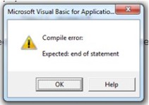
Note that normally the message box code would all be on one line or perhaps on a couple of lines with an underscore (line continuation marker) at the end of line 1.

If you are unsure about how message boxes work refer to my blog Excel VBA Message Boxes ( http://wp.me/p2EAVc-3 )for more information.

So that is one simple application of the FOR…NEXT type loop. How about scrolling through a bunch of cells?

Looping through a range of cells;

Let’s say I have some data and I want to apply a bit of formatting. I could create a DO UNTIL type loop moving from row to row and then column to column, but a FOR…NEXT loop will be far more efficient.

I want to highlight all cells with a value under 100 by making the font red. I need code that will select the entire table, and then check each cell to see if each cell is under 100 and change values to a red font.

Dim c as Range   ‘create an object variable to represent each cell in the selected range

Range(“A1”).CurrentRegion.Select  ‘(selects all contiguous cells around A1)

For Each c in Selection

          If c.Value <100 then ‘(tests if the value in each cell is less than 100)

                   c.Font.Color = vbRed

          End If

Next c ‘(loops through all cells in the selected range until it runs out)

So this is much easier than trying to work out when to go back to the top of a column and then move across one and so on and so forth.

Below is a video showing a For Each…Next loop in action showing how to use the IMMEDIATE WINDOW to find out what the code is doing and where.

Looping through multiple sheets;

I can apply the same logic to any number of sheets in a workbook.

Dim Ws as Worksheet

For Each Ws in ActiveWorkbook.WorkSheets

If WorksheetFunction.Counta(Ws.Cells) = 0 Then
‘(test if all cells are blank/empty)

                   Ws.Delete

          End If

Next Ws

So how does this work?

First we need an object variable (Ws) to represent any worksheet in the workbook. This is needed because we don’t necessarily know how many worksheets are in the current workbook or what they are called, so we need a way of referencing each sheet without being specific (i.e. hard coding names/numbers). And this is one of the issues you will have if anything goes wrong. The worksheet you are in is the active sheet, but you never move away from it. All the movement from sheet to sheet happens in the background, so in STEP INTO DEBUG mode you can’t see which sheet is being tested at any point while the macro is running. You have to rely on the IMMEDIATE WINDOW. To open the IMMEDIATE WINDOW select it from the VIEW menu or press CTRL + G.

The IMMEDIATE WINDOW lets you question the VB EDITOR. The only downside to this is you have to ask the questions in VBA! So, to find out which sheet is currently being checked the code above you would need to ask;

?Ws.Name

Remember you cannot ask about the ActiveSheet as it is always the same one – whichever sheet you started in.

Looping through multiple workbooks;

Having seen how to loop through multiple worksheets, this logic can be extended to do the same with multiple workbooks.

Dim Ws as Worksheet, Wb as Workbook

For Each Wb in ActiveWorkbooks

          For Each Ws in Wb.Worksheets

                   If WorksheetFunction.Counta(Ws.Cells) = 0 Then

                             Ws.Delete

                   End If

          Next Ws

Next Wb

Now we have one object variable for the worksheets and one for the workbooks. The code will look for any open workbooks, and for each one it finds it will scroll through all the worksheets to see if they are blank or not and then move on to the next open workbook until it runs out of workbooks to check. By using object variables there is no need to hard code names etc. relating to the open workbooks or worksheets. Remember, if you need to check which workbook or worksheet is being checked by the code you will need to do this in the IMMEDIATE WINDOW.

One word of warning: if PERSONAL.XLSB is open it will treat it as an open workbook and test its sheets too. Problem is PERSONAL.XLSB only has one sheet and it is blank as this workbook is never used other than to write code to. If the code tries to delete its one and only worksheet it will crash as workbooks cannot exist without any worksheets. To get around this you need an IF statement before starting the loops to test the name of the current workbook.

So there you have the basics of loops in VBA:

• DO UNTIL/WHILE…LOOP
• FOR…NEXT

Both have their uses. DO loops tend to be easier to create and test, but FOR…NEXT loops are more efficient but tend to require object variables to get the most out of them and are a little trickier to test using the IMMEDIATE WINDOW.

It’s now down to you to put these into practice and apply them to whatever project you are working on.

Excel VBA – Looping Part 1

One thing you cannot record as part of an Excel macro is looping i.e. moving from one row/column, worksheet or even workbook to another. You can record copying a formula down a column or similar, but it records it as AUTOFILL and therefore records the cells as absolute references meaning that if you have any variation to the number of rows etc. when you recorded the macro, it won’t work properly. So this is where you need to do LOOPS in VBA.

There are two basic loops you can use;

• Do While/Until…..Loop
• For each…..next

In this first blog I am going to go through the DO WHILE/UNTIL type loop.

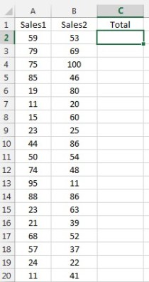
Let’s take a simple example, where I want to add a formula in column C adding up values in columns A and B.

 

Simple table to add a formula column to

The code required to do this would be as follows;

First we need a start point i.e. where do we want to start the loop from? In this example, the first cell is C2.

Range(“C2”).Select

or

Cells(2,3).Select (use whichever method you prefer)

Then we need to give an instruction when to stop looping. Here, we want the code to stop running when the cell(s) to the left of the formula cell is/are empty. You would need to decide how to handle this depending on the data you have – are all columns full of data? Are there any blanks in either or both columns? This will determine what you need to put in your DO UNTIL/WHILE command.

Do Until ActiveCell.Offset(0,-1).Value = “” (stop when cell to left is blank)

Or

Do Until Activecell.Offset(0,-2).Value = “” And ActiveCell.Offset(0,-1).Value = “” (stop when both columns A and B are blank)

If you are not familiar with the OFFSET function in VBA, it allows you to reference cells based on their distance in terms of ROWS and then COLUMNS from the selected or active cell.

Positive numbers refer to ROWS down and COLUMNS to the right, whereas negative numbers refer to ROWS up, and COLUMNS to the left of the active cell. If you had cell C5 selected, for example, then;

ActiveCell.Offset(2,-1) would refer to cell B7 – two rows down & 1 column to the left.

The alternative to DO UNTIL is DO WHILE. Works the same way, just a question of logic to tell the code when to stop. If using DO WHILE in our original example the code would be like this;

Do While ActiveCell.Offset(0,-1)<> “” (keep going as long as the cell in the column to the left is not empty)

Personally, I tend to go with DO UNTIL…seems more logical to me, but the choice is yours.

Get into the habit of adding in the word LOOP to make sure you close off the pairing of code words. This will give us the following code so far;

Range(“C2”).Select

Do Until ActiveCell.Offset(0,-1).Value = “”

Loop

One thing you will always need in a LOOP, is movement. You need to add a line that tells the editor which direction to travel in as part of the loop. If you don’t do this, then you stay permanently in the start cell and therefore in a permanent loop. If that happens you can use CTRL + BREAK to stop the loop and show the END/DEBUG window. If it is the LOOP causing the problem the code word LOOP should be highlighted in yellow.

In this example, I need to move down a row each time so I will add the line;

ActiveCell.Offset(1,0).Select

This should be just above the LOOP line. If you go on to do more complex loops, think carefully where the movement comes in. I’ll show you a simple example later.

The final part of the code is to tell the code what to do with each loop. In this example it is to add a formula. Here, I will be using R1C1 cell referencing style. If you don’t know what that is, or how it works check out my blog about R1C1 reference style ( http://wp.me/p2EAVc-4I ). Good to know when it comes to VBA formulas!

My final code will therefore be;

Range(“C2”).Select

Do Until ActiveCell.Offset(0,-1).Value = “”

          ActiveCell.FormulaR1C1 = “=SUM(rc[-2]:rc[-1])”

          ActiveCell.Offset(1,0).Select

Loop

When you have a loop set up, it’s always worth a look step by step using the DEBUG tools to see the loop in action and to check that it’s doing everything it’s meant to be doing, especially if any variables are concerned.

I mentioned earlier about being careful where you put your movement line in your code. Let’s take a look at a bit of code that removes blank lines from a worksheet;

Range(“C2”).Select

Do Until ActiveCell. Value = “End”

          If ActiveCell.value = “” then

                   Rows(ActiveCell.Row).Delete

          Else

                   ActiveCell.Offset(1,0).Select

          End if

Loop

Here, the movement is built into the IF statement, rather than at the end just before the LOOP. This is necessary because when you delete a row, all rows underneath automatically move up to “fill the void”. If you move each time you delete a line, and there are two or more blank rows in succession, the next blank row would move up to your current location, and then the cursor would move down a row, completely missing out testing the row that had just moved up. The video below will show clearly what happens if the movement is just before the loop, and then with the movement in the IF statement.

So there you have some basic code to create a loop. Looping Part 2 will look at the FOR EACH…NEXT type loop which is a quicker and more efficient way of looping, letting you loop through multiple worksheets and workbooks in seconds, but do get used to the DO UNTIL/WHILE loop. It has its uses and is easier to debug and test than the FOR…NEXT type loops as you will see in Part 2 of looping.

Excel VBA – Copying & Pasting

Cut, copy, paste must be the bane of some people’s working lives. Whether you use right clicks or keyboard shortcuts to do it, chances are this is one of the most common repetitive actions you do at work, whether it is in Excel, Word or pretty much any application you care to think of.

A large proportion of what we copy and paste will be one off events, but those of you who do monthly reporting, or any type of reporting for that matter, you probably find yourself doing a lot of copying and pasting of the same data, month after month.

In this blog I will show you some simple code that will automate the whole process. I will break this down into sections;

• Within the same worksheet
• Between different worksheets
• Between different workbooks
• Using the clipboard
• Using paste special

Copy/Paste in the same worksheet

Basic sample data

We have some data in cells A1:A11 and want to copy it across to another part of the same worksheet. For this example, let’s say I want to start pasting the data starting from cell E12.

Let’s just think about how we would do this manually first – highlight the cells A1:A11, right click, select COPY or press Ctrl + C, click into cell E12 and press Ctrl + V or right click and select PASTE. I don’t need to select a range of cells to paste into, just pick the top left hand cell to start pasting from.

It’s exactly the same in VBA:

Say what you want to copy, what you want to do to it i.e. copy and tell it where to start pasting from.

Range(“A1:A11”).Copy Range(”E12”)

Note, I do not need to use the word PASTE anywhere in my code. By keeping all the code on ONE line, the cell reference that follows the space after COPY is the DESTINATION cell to start the paste operation from.

The key to keeping this simple is to ensure the copy/paste instructions are kept on the same line. If you move to a second line of code, the data is stored in the CLIPBOARD and has to be extracted again. I’ll show this a bit later but most of the time it is unnecessary.

If you want to CUT and PASTE then replace the word COPY with CUT – simple as that!

This code assumes that we are copying and pasting within the ActiveSheet. If we want to be a little more precise to avoid any errors then we can specify the name of the worksheet we want to copy and paste in;

Worksheets(1).Range(“A1:A11”).Copy Range(“E12”)

By being that little more specific we don’t have to worry too much about which worksheet we are in when the code runs. We can be even more specific by naming the workbook too and that avoids any issues of current workbook or current worksheet.

Workbooks(“Demo”).Worksheets(1).Range(“A1:A11”).Copy _ Range(“E12”)

In keeping with writing code I have used a space followed by an underscore as a continuation marker. This tells the VB editor that this is a continuous line of code and not two separate lines. This is useful when you write code as it means you do not have to keep on scrolling across to the right to read a long line of code…particularly handy when writing long lines of code for copy/paste!

Copy/Paste between different worksheets

Basically you need to reproduce what we did in the example above only now you have to specify a source sheet and destination sheet. Think of it a bit like an equation that needs to be balanced either side of your copy/cut command;

Worksheets(1).Range(“A1:A11”).Copy Worksheets(2).Range(“A1”)

As in the previous example I can be a little more precise by naming the workbook at the beginning just in case I don’t happen to be in the workbook when the code is running.

Copy/Paste between different workbooks

Same again, but this time I need to make sure I reference the source workbook name and the destination workbook name as well as the sheet and range references;

Workbooks(“Source”).Worksheets(1).Range(“A1:A11”).Copy _

Workbooks(“Destination”).Worksheets(2).Range(“A1)

Remember to keep the code on one continuous line or use the line continuation marker ( _).

When using the CUT/COPY code, because you can be very precise with the workbook, worksheet and range references, as long as those workbooks are open you don’t have to make either one of the workbooks active. The code will run irrespective of which workbook you are in, making this code very efficient as you don’t have to activate or select anything for it to work.

Move/Copy/Paste entire worksheets

Rather than just CUT/COPY a range of cells, you may want to do it to an entire sheet.

Virtually no difference with the code above, only now we don’t need to reference the cells, only the worksheet.

Worksheets(1).Move Worksheets(3)

Worksheets(1).Move ,Worksheets(3)

The first line will move sheet 1 to the LEFT of worksheet 3 and the second line of code, the addition of the COMMA moves the sheet to the RIGHT of worksheet 3. You could of course COPY the sheet instead…works exactly the same way.

The make the code a little clearer you can use the word BEFORE:= or AFTER:= rather than no comma, or comma respectively to place the worksheet.

Similar to copying cells between workbooks, you have to specify the source and destination workbooks.

Workbooks(“Source”).Worksheets(1).Move _ Workbooks(“Destination”).Worksheets(1)

The absence of a comma after MOVE will place the worksheet to the LEFT of sheet 1 in the destination workbook, and a comma will move it to the RIGHT.

Note there is no reference made to cells. When you copy or move an entire sheet you cannot paste it into a cell or range of cells unless you copy all the cells in a sheet rather than the sheet itself. It’s a bit like tearing a sheet out of a book…you don’t stick it on top of a sheet covering what is already there, you slide it in before or after an existing sheet.

Copying to the clipboard

There may be times when you don’t want to CUT/COPY/PASTE immediately to a known destination as you may need to do some work first in a sheet and paste some information below it.

Range(“A1:A11”).Copy

…do whatever else needs doing with your code

ActiveSheet.Paste

Application.CutCopyMode = False

Unlike the earlier examples the COPY and PASTE actions are now two separate lines of code. When you COPY it is put on the clipboard. Eventually you will be in an ActiveCell and that is where you use the ActiveSheet.Paste command. The final line above is used to clear the clipboard.

Note that this method only allows you to copy one thing at a time to the clipboard. There are ways of working with multiple items but it’s beyond the scope of this blog.

Using Paste Special

If you are used to Excel 2010 or 2013 you will know how easy it is now to access the features of Paste Special. To write this in VBA is not that difficult.

Pick list showing options for Paste Special

Copy your cells exactly the same as before, go to another cell, same sheet/same workbook/other workbook and use the .PasteSpecial command followed by a bracket. When you type the bracket you will see the prompt to show all the parameters and the first one is the paste TYPE. Choose from:

• xlPasteAll
• xlPasteAllExceptBorders
• xlPasteAllMergingConditionalFormats
• xlPasteAllUsingSourceTheme
• xlPasteColumnWidths
• xlPasteComments
• xlPasteFormats
• xlPasteFormulas
• xlPasteFormulasAndNumberFormats
• xlPasteValidation
• xlPasteValues
• xlPasteValuesAndNumberFormats

You then have two more optional parameters you can set;

Special operation:

• xlPasteSpecialOperationAdd
• xlPasteSpecialOperationDivide
• xlPasteSpecialOperationMultiply
• xlPasteSpecialOperationNone
• xlPasteSpecialOperationSubtract

And finally, decide whether you want to SKIP BLANKS or not. Set this parameter to TRUE or FALSE.

You can use the CutCopyMode line of code again to clear the clipboard and remove the dashed lines (2013) or the marching ants around the copied cells.

The one option that is missing from here is PASTE LINK.

Follow the code to do COPY and PASTE using the clipboard but on the PASTE line of code add a comma and TRUE. This will then paste in as a link.

ActiveSheet.Paste, True

Note that you will not be prompted with anything when you enter the comma…you just have to know.

So there you have CUT/COPY/MOVE/PASTE/PASTESPECIAL/PASTE LINK in VBA for Excel. No more manual cut/copy/paste on those monthly reports!

Interactive Excel Voting Board

If you run a training session, or perhaps you chair a meeting, you want to get some instant feedback, or perhaps you want attendees to vote on something. You can do a simple show of hands which works fine, but how about something a little more high tech but without going overboard?

Ideally, for this to work, and in particular to get people involved you will need a touch screen. You could just use a mouse on the computer but this seems to work quite well and gets people out of their seats participating in the session.

There are two ways I can do this:

• The non VBA way
• Using VBA

Let’s start with the non VBA way using FORM CONTROLS.

If you are using 2003 then you will need to activate your FORMS toolbar. Go to VIEW, TOOLBARS and select FORMS. Do not use CONTROL TOOLBOX which looks very similar as this requires the use of VBA to make things work.

If you are using 2007 or later, turn on the DEVELOPER tab and you will find FORM CONTROLS under INSERT in the CONTROLS group.

Select the SPIN BUTTON option. Your cursor will change to a small cross-hair. Click and drag somewhere in your worksheet to “draw” the SPIN BUTTON. You can move and resize this at any time if it’s not quite right so don’t worry if it does not look quite right yet.

Right click on the new SPIN BUTTON and select FORMAT CONTROL.

In the dialog box decide what your minimum and maximum are and also the increment that each click of a button will increase/decrease the value by. So in this example I will set the minimum to 0, the maximum to 10 and the increment value to 1.

The final thing you need to set is a reference cell or CELL LINK. The form controls do nothing other than look pretty. In order for them to work, you have to link them to a cell and it is this cell that will do the work.

Click on OK.

Now create a chart based on the value in the CELL LINK.

Format your chart whichever way you want and repeat as many times as necessary to create multiple charts to display people’s votes.

Now for the VBA version. If you are familiar with VBA then this is a very simple way of doing things, and if you aren’t familiar then this is simple enough to have a go.

The benefit of VBA over the FORM CONTROLS is you have more options available to you and you can, if you want to, go mad and program it to do all kinds of weird and wonderful stuff…but for now, here is a simple example for you which you can embellish as your VBA skills grow.

This time start by entering the value 0 in a cell.

Now add a button to the worksheet, but this time use the ACTIVE X CONTROLS, NOT the form controls we used in the previous example.

Click on the BUTTON icon then click and drag to “draw” a button on the worksheet. Again this can be moved at a later stage if it’s not in the correct position.

Click on the PROPERTIES button and do the following:

• Give a suitable name to your button (helps when writing code)
• Enter a caption i.e. what you want to display on the button face

There are many more options you can go for but this would be the bare minimum at this stage.

Close the PROPERTIES window for now.

Now we need to add some code to our button to make it work. Double click the newly added button, making sure that you are in DESIGN mode in order to be able to make changes to your button.

 

I declare a PRIVATE variable in my GENERAL DECLARATIONS area at the top of my code sheet. I need this to store the value of the cell that I am associating with the button and subsequent chart.

I can then add the following bit of code:

 

Again, repeat as many times as necessary to build up your voting board.

So far though, we only have a button that increases the value of the cell. We now need to add one that takes the value down by one each time we click on it. At this point you are probably thinking that this is a bit long winded, considering we had a single button that did both before. Using this method means you can have a more customised look and feel to your voting board rather than just up/down arrows (the choice is yours!)

Follow the same steps as before to add a new button and then add the following code:

 

This time as well as decreasing the value of cell C6, I have added an IF statement to prevent negative values from being generated.

The final button you might want to add is reset button so you can quickly reset the value(s) to 0. This might be worth doing last of all once you have created all the voting buttons and charts you need and then have a single button to reset all the reference cells in one hit

.

 

Simply add extra cell references once you have set them all up e.g. Range(“C6, F6, I6”).Value = 0

Your final interactive voting tool will look something like this…

 

So next time you want to have a poll in class or at a meeting you can do it with a little more style than just a show of hands.

Excel – R1C1 Reference Style vs. A1

If you have ever strayed into the Options screens of Excel you may have noticed something called R1C1 reference style. You may have even tried it and when you saw that all the columns had changed from letters to numbers, panicked and switched it back.

However, the R1C1 style has some advantages over the standard A1 style, but it does take a bit of getting used to!

So is this R1C1 style new? Well in fact not at all. This cell reference style dates back to 1982 and the introduction of Multiplan as a rival to VisiCalc and Lotus 1-2-3. Multiplan was developed by Microsoft for Apple Macintosh and used this cell referencing style instead of what was to become the standard in spreadsheets – A1 style.

Over the next few years, Lotus 1-2-3 became “the” spreadsheet package. In order for Microsoft to steal Lotus users who were used to the A1 style they added the A1 style to Excel so that people who migrated across would find it familiar. Excel eventually overtook Lotus in 1993 as the industry standard for spreadsheets. The rest as they say is history.

But enough of the history lesson…how does R1C1 differ to A1?

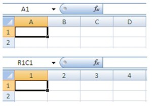
The most obvious difference is the column references. Instead of letters you get numbers.

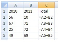
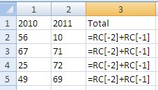
The real difference comes when you want to write formulas. Let’s take a simple example adding two columns together. I am displaying the formulas so the differences are clearer.

First, the familiar A1 style:

And now for R1C1….

At first this looks quite horrific and ten times more complicated that the A1 style. Before I break down how it works, what do you notice between the two styles (other than the obvious one)?

Each formula is different in A1 style: A2+B2, A3+B3…etc.

Whereas using R1C1, they are all identical. So this potentially means that wherever you write a formula in that column it will be same, no need to think about which row or column you are in. This is particularly helpful when you are writing VBA code.

So how does it work?

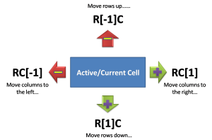
Any numbers in square brackets refer to relative distance from the current cell. Unlike A1 which refers to columns followed by row number, R1C1 does the opposite: rows followed by columns (which does take some getting used to).

Positive numbers will refer to cells below and/or across to the right.

Negative numbers will refer to cells above and/or to the left.

For example R[2]C[3] is a cell 2 rows down and 3 columns to the right. R[-1]C[-4] is a cell 1 row up and 4 columns to the left. If no number is shown in brackets then you are referring to the same row or column i.e. R[3]C will be a cell 3 rows below the current cell in the SAME column.

So once you have the basics, they are actually not that bad. Note however, that you cannot use an A1 formula when displaying R1C1 style and vice-versa. Whichever system you use, Excel ‘translates’ the styles should you switch between them at any point.

The other difference between the two styles is absolute referencing. In the A1 style I need to add $ symbols all over the place. Granted I can use F4 to put them in place for me but it still needs to be done. In R1C1, there are no $. If I write R3C4 I am referring to $D$3. So if there are no brackets, it’s an absolute reference. This makes partial absolute references easier to enter too.

The R1C1 style definitely does have some neat advantages over A1, but we are so used to the A1 style that moving away from it is an alien concept. But if you ever have a chance, try playing with R1C1, especially if you progress to VBA, and I can guarantee that writing formulas will become a lot easier…the pain is only short-lived but it is worth the effort.

For a bit of further reading on R1C1 follow this link (http://tduhameau.wordpress.com/2012/09/27/the-beauty-of-the-r1c1-reference-style/)

Excel – Create Your Own Custom or User Defined Function (UDF)

As we all know Excel has more built in functions than any one human could ever need. Personally I have never had to use the BESSELK function and I very much doubt I ever will….in fact I have no idea what it does.

But what if there is some sort of calculation you do on a regular basis for which there is no built in function? You may well have a calculation that is specific to your company or job role and you use it on a daily basis. The calculation itself might be quite complex and requires lots of brackets, sub-calculations etc making it prone to typing errors or simply takes you ages to put together each time you need it.

What if you could create your own function with all the calculations built in and all you had to do was enter the basic data? Well…you can, with the help of VBA.
First of plan your function on paper; what is the calculation going to do and how?

For each element within your calculation, how many variables do you have? This is where it gets a bit confusing for people not used to working with or even knowing what I am referring to as variables.

Let’s try and build a simple example to understand what a variable is and how we can build variables into our function.

I want to be able to calculate the cost of a car journey so I can work out costs more accurately rather than just apply a flat rate per mile.

So what would I need to know to work this out?

• The distance driven

• The cost of fuel

• The average fuel consumption of the car being used to make the journey

Of these three values I need, how many will vary each time I need to do the calculation?

• Each journey will be different so the mileage will vary each time

• The cost of fuel is always changing (usually upwards!)

• Unless you only have one pool car, chances are you will be using different cars, each with their own fuel consumption rate

These are VARIABLES. In each case, there is no fixed value whenever we come to do the calculation. Hopefully, that clears up what a variable is.
So our calculation might be;

(distance driven/fuel consumption) * (cost of fuel * 4.5)

The *4.5 bit is more of a UK thing….fuel prices are quoted as cost per litre but we base fuel consumption on miles per gallon, and one UK gallon is 4.5 litres.
If we were to put numbers into this we might have;

(200miles/35mpg)*(£1.41 per litre * 4.5 litres) = £36.26
i.e. the cost of fuel to do a 200 mile journey in a car that does 35 miles per gallon.

Now that we have planned our function on paper, we now need to translate it into VBA code. Make sure you have a blank workbook open.

Go to the DEVELOPER tab and click on VISUAL BASIC, or press CTRL + F11. If you use 2007 or 2010 it may not be visible. For 2007 users, go to the OFFICE button, select EXCEL OPTIONS and on the POPULAR tab tick SHOW DEVELOPER TAB IN THE RIBBON. If you are on 2010, right click in the ribbon and select CUSTOMIZE RIBBON and tick the DEVELOPER option.

Remember earlier on in this task we opened a blank workbook? In the project window you should see something like VBAProject(Book1). Right click on the name of the workbook (project in VBA terms), click on INSERT, then click on MODULE. A MODULE is simply a folder that stores code within the workbook.

You should now have a blank page to the right of the project explorer window…that’s the list of open workbooks on the left hand side.

Now I need to declare my variables by giving them a name and data type.

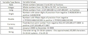
The data type you use is important when working with variables. Each variable can only store one type of information. The basic variable types you are likely to use are as follows:

There are others but if you know these it’s a good start.

All that’s left now is to create the function itself substituting the names of the variables into our formula. Start by using the name you have given to your function (make sure you do this or your function won’t work);

If you are not used to working with variables, this does seem a bit odd to start with, looking at a formula that contains words rather than numbers.

To test your new function start typing the name in a cell (in the same workbook that contains the code module) where you want to perform the calculation;

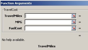
The new function appears in the pop up list of functions! If you cannot remember the order of the variables you need to enter to make the function work, click on the fx button next to the formula bar. This will show you the wizard for your function, showing each variable you need to add in.

Use the wizard as you would any normal function and hey presto…you have an answer without the need to type out all the brackets, constants, operators etc.

If you are happy with your new function and want to make it a permanent part of YOUR Excel you need to save the workbook containing the code as an ADD-IN.

Make sure the workbook is clear: no calculations or data in the workbook. Then just do a SAVE AS, selecting EXCEL ADD-IN(*.XLAM), name the workbook, ideally using the function name and click on SAVE.

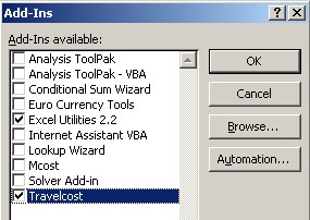
To make the function available in Excel you need to activate the add-in. Go to the OFFICE button (2007) or FILE (2010), then click on EXCEL OPTIONS, and then ADD-INS.

At the bottom of the window make sure EXCEL ADD-INS is showing and click on GO.

Tick your newly saved function as an add-in, and click on OK. You are now free to use your function whenever you want in any workbook on your laptop/PC. So if you are some sort of budding quantum physicist or you just have a special way of calculating your home finances, you can now put your own functions into Excel to work on all your data.

 

Excel VBA Message Boxes (Part 3)

In my earlier blogs we looked at how to customise the overall appearance of a message box and then on how to customise the message itself. This time let’s look at how we can interact with the message box by performing different actions based on the button selected.

When you first set up a message box with multiple buttons, whichever one you click on will do exactly the same i.e. close the message box. This of course is of no use to anyone.

Each button, however, has a value assigned to it (or 2 to be precise). This can be a system constant or a numerical value.

The values for each button are as follows:

I have not added the ‘OK only’ option for obvious reasons!

Once we know that each button has a value, we can use this to write code so that if the user selects ‘Yes’ we can make it do one thing and something else if they select ‘No’.

In order to store the value of the selected button we need to create a variable, making sure that the variable type matches the value you are storing. In this example I am going to use byte as my data type, as we are dealing with whole numbers with a maximum value of 7 (well below the 255 maximum a byte can handle).

So our code would look something like this:

Sub RespondToMessage()

Dim Reply as Byte

Reply = MsgBox (“Please select a button”, vbYesNoCancel + vbQuestion _ ,“Respond”)

Select Case Reply

          Case Is = 6

MsgBox “You selected ‘Yes’”, , “Well done!”

          Case Is = 7

MsgBox “You selected ‘No’”, , “Well done!”

          Case Is = 2

 MsgBox “You selected ‘Cancel’”, , “Well done!”

End Select

End Sub

Ok…not the most useful set of instructions once you’ve clicked on a button but you get the idea. You can make the response to any button as simple or as complex as you like.

Note: when we state what the variable is equal to we have to add brackets around everything that goes into the message box, including any options and custom titles. If you don’t do this you will be prompted with an error message.

In this example I have used Select Case but you could equally use an If Then Else/If ElseIf Then type statements.

This is a great way to make your macros more interactive by giving the user options as the code runs; Do you want to print the modified sheet? Have you checked the printer for letter headed paper? Etc…etc…the possibilities are endless.

Follow me on Twitter @excelmate